Published on: 2026-03-27
Updated on: 2026-07-06
The Black-Scholes model gives traders a way to estimate an option’s theoretical value rather than relying solely on the market premium. The growth of listed options trading has also increased the importance of understanding how Option premiums are priced.
U.S. listed options volume reached a record 15.2 billion contracts in 2025. SPX 0DTE options also averaged 2.3 million contracts daily, equal to 59% of total SPX options volume. In this environment, a clear formula, calculator, and pricing example help explain what an option premium really reflects.
The Black-Scholes model estimates the theoretical price of European call and put options.
Its main inputs are the underlying price, strike price, time to expiration, risk-free rate, and volatility.
Volatility often has the largest impact because it changes the expected price range.
The model works best as a benchmark, not as a perfect prediction of market prices.
Its limits matter most around dividends, early exercise, liquidity gaps, event risk, and 0DTE options.
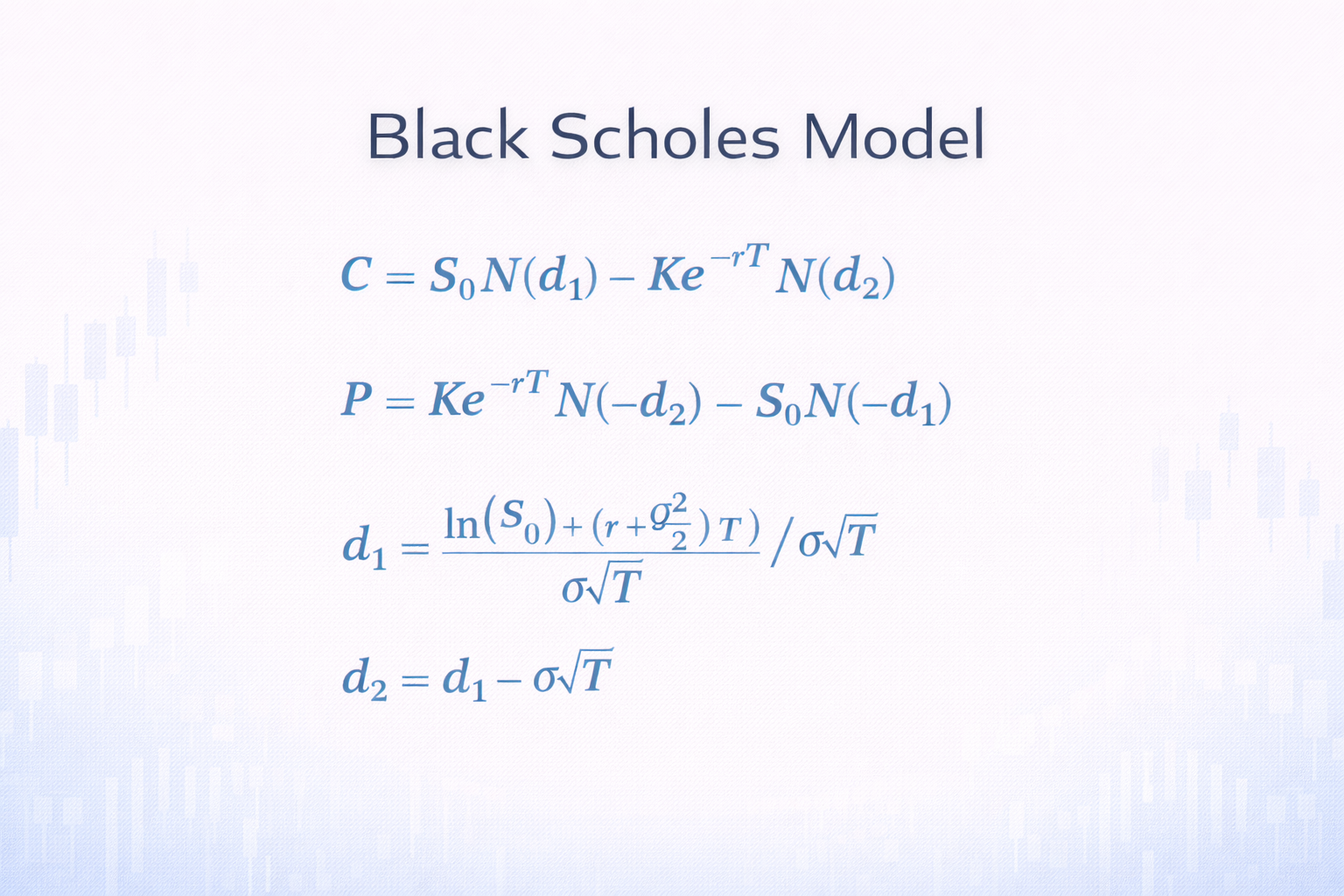
The Black-Scholes model is an options pricing model developed by Fischer Black, Myron Scholes, and Robert Merton in the early 1970s. It estimates an option's value today based on the asset price, strike price, time to expiration, interest rates, and expected volatility.
The standard model applies to European options, which can only be exercised at expiration. American options, which can be exercised early, often require adjusted models.
The model does not say whether an option will be profitable. It gives a theoretical fair value that traders can compare with the market price.
The Black-Scholes model helps traders answer practical questions such as:
Is an option expensive or cheap relative to implied volatility?
How much value comes from time rather than intrinsic value?
How sensitive is the option to price, volatility, and time decay?
How much does the option’s theoretical value change if market conditions change?
For many traders, the model is less about predicting price and more about understanding what the market premium already reflects.
For a European call option, the Black-Scholes formula is:
C = S × N(d1) - K × e^(-rT) × N(d2)
For a European put option, the formula is:
P = K × e^(-rT) × N(-d2) - S × N(-d1)
The probability terms are:
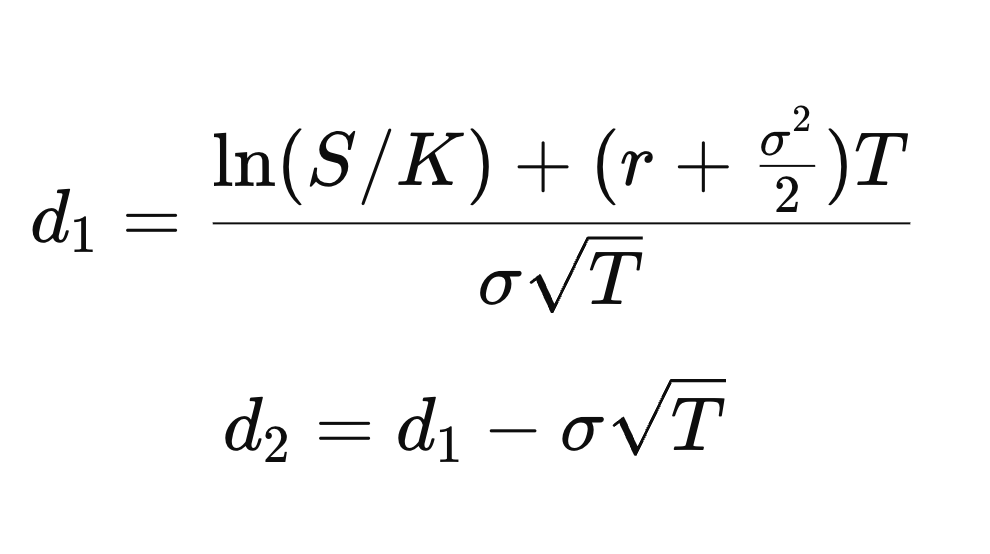
d1 = [ln(S/K) + (r + σ²/2)T] / [σ√T]
d2 = d1 - σ√T
Using these variables, the price of a European call option is calculated as:
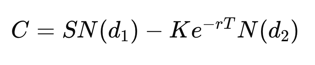
Where:
C: Theoretical call option price.
S: Current price of the underlying asset (spot price).
K: Strike price of the option.
r: Risk-free interest rate (annualized).
T: Time to maturity (in years).
σ (sigma): Volatility of the underlying asset's returns.
N(d₁), N(d₂): Cumulative distribution function of the standard normal distribution.
e^{-rT}: Discount factor for present value.
d₁: The delta of the option, representing the sensitivity of the option price to changes in the underlying asset's price.
d₂: The probability that the option will expire in the money.
S × N(d₁): The expected benefit from receiving the stock, contingent on exercise.
K × e^{-rT} × N(d₂): The present value of the cost to exercise the option, contingent on exercise.
For a European put option, the formula is:
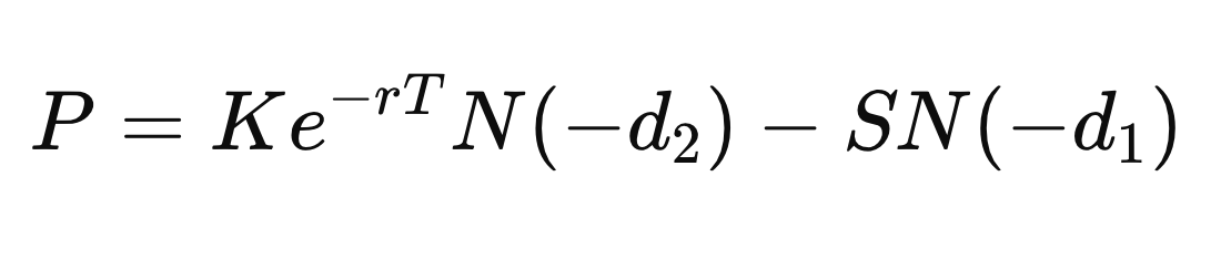
The formula separates the option value into expected gains and discounted costs. Volatility plays a central role because it increases the probability of favourable price movements, which raises the option’s value.
Consider a trader evaluating a call option on a stock trading at 100 dollars with a strike price of 105 dollars and three months to expiration.
If volatility is low, the probability of the stock exceeding $ 105 is lower, so the option will be cheaper. If volatility increases, the likelihood of a profitable outcome rises, which increases the option price.
By applying the Black-Scholes model, the trader can estimate a fair value and compare it to the market price. This allows for more informed trading decisions.
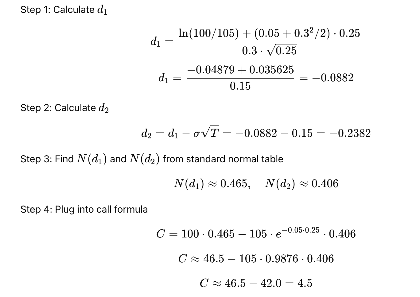
Call option theoretical price = $4.50
This tells the trader that paying more than $4.50 may be overpriced, while paying less may represent an opportunity.
An interactive Black-Scholes calculator should sit directly below the formula section. Readers should be able to enter the core inputs and immediately see the estimated option price.
Calculator Input |
Example Value |
Option type |
Call |
Current asset price |
$100 |
Strike price |
$105 |
Days to expiration |
90 |
Risk-free rate |
3.75% |
Volatility |
30% |
Dividend yield |
0% |
The calculator should show estimated option value, intrinsic value, time value, delta, gamma, theta, vega, rho, and moneyness.
The output is a theoretical value, not a trading recommendation. Market prices can differ due to liquidity, dividends, earnings, volatility skew, and supply-and-demand pressures.
Assume a $100 stock. A trader wants to price a three-month European call option with a $105 strike, 90 days to expiration, a 3.75% risk-free rate, and 30% volatility.
| Input | Value |
|---|---|
| Stock Price | $100 |
| Strike Price | $105 |
| Time to Expiration | 90 days |
| Risk-Free Rate | 3.75% |
| Volatility | 30% |
| Estimated Call Value | $4.25 |
The option is out of the money because the strike price is above the stock price. Yet it still has value because there is time for the stock to move above $105 before expiration.
If the market price is $5.50, the option trades above the model value. That may mean implied volatility is rich, or that the market expects a larger move than the model inputs assume.
If the market price is $3.50, implied volatility may be lower than the model assumptions, although liquidity, dividends, event risk, and market conditions can also explain the difference.
For the same inputs, the estimated European put value is about $8.29. The put is more expensive because a $105 strike put already has intrinsic value when the stock trades at $100.
The model combines probability, discounting, and volatility. A call option becomes more valuable when the underlying price rises, volatility increases, or more time to expiration remains. It becomes less valuable when the strike price is higher or time decay accelerates near expiry.
| Input Change | Call Option Impact | Reason |
|---|---|---|
| Stock Price Rises | Increases | More chance of finishing in the money |
| Strike Price Rises | Decreases | Exercise becomes harder |
| Time Increases | Usually Increases | More possible price paths |
| Volatility Rises | Increases | Wider price swings raise option value |
| Risk-Free Rate Rises | Usually Increases | The strike price is discounted more heavily |
Volatility usually has the biggest impact on option pricing. A stock can stay flat while its options rise if implied volatility increases. A correct directional view can still lose money if volatility falls sharply after an event.
In listed options, traders compare market premiums with theoretical value. If an option trades above model value, implied volatility may be expensive. If it trades below model value, implied volatility may be lower than the assumptions used in the calculation.
Portfolio managers use the model to estimate hedge costs. A protective put can be priced across different strikes and expirations to compare protection levels.
Market makers use Black-Scholes as a base for quoting options and managing Greeks. Delta tracks price sensitivity. Gamma measures how quickly delta changes. Theta captures time decay. Vega measures volatility exposure. Rho measures rate sensitivity.
Companies also use option pricing models to value employee stock options. Even an out-of-the-money option can retain value because time and volatility create the possibility of future profit.
The model depends on simplified assumptions:
The option is European-style.
The underlying asset follows a lognormal price path.
Volatility and the risk-free rate are constant.
There are no transaction costs.
Markets are liquid and allow continuous trading.
The original model assumes no dividends.
There are no arbitrage opportunities.
These assumptions make the model fast and useful. They also explain why market prices often differ from theoretical values.
The biggest limitation is constant volatility. Real markets have volatility smiles, skew, and sudden repricing around earnings, inflation data, central bank decisions, and geopolitical shocks.
The model also struggles with early exercise. This matters for American options and dividend-paying stocks, where exercising before expiration can sometimes make economic sense.
0DTE options create another challenge. Gamma can rise sharply as expiration approaches. A small move in the underlying asset can quickly change delta, hedge demand, and theoretical value.
Liquidity also matters. An option may look cheap in theory, but a wide bid-ask spread can erase the advantage.
| Model | Best For | Strength | Limitation |
|---|---|---|---|
| Black-Scholes | European options | Fast benchmark pricing | Assumes constant volatility |
| Binomial Model | American options | Handles early exercise | More complex |
| Monte Carlo Model | Exotic options | Models many scenarios | Computationally heavy |
Black-Scholes is often the starting point. Binomial models are better when early exercise matters. Monte Carlo models are more useful for complex options with multiple variables or path-dependent payoffs.
It estimates the theoretical value of European call and put options. Traders also use it to calculate implied volatility, compare premiums, understand Greeks, and assess whether market pricing looks rich or cheap.
The formula needs the current asset price, strike price, time to expiration, risk-free rate, and volatility. Adjusted versions may also include dividend yield for dividend-paying stocks.
The standard model is designed for European options. American options can be exercised early, so traders often use binomial or adjusted models when dividends or early exercise affect value.
Volatility measures expected price movement. Higher volatility increases the chance that an option finishes in the money, thereby raising the theoretical value of both calls and puts.
Yes. It remains a core benchmark for options pricing, implied volatility analysis, hedging, and risk management. Traders often adjust the model to account for real-world factors such as dividends, volatility skew, liquidity, and early exercise.
The Black-Scholes model remains central to options pricing because it links price, strike, time, rates, and volatility into one clear estimate of theoretical value.
Its assumptions are imperfect, especially in markets shaped by 0DTE trading, volatility skew, dividends, and event risk. Still, the model remains the essential starting point. A formula breakdown, calculator, and pricing example make it easier to see what an option premium really represents.
Disclaimer: This material is for general information purposes only and is not intended as (and should not be considered to be) financial, investment or other advice on which reliance should be placed. No opinion given in the material constitutes a recommendation by EBC or the author that any particular investment, security, transaction or investment strategy is suitable for any specific person.