Published on: 2026-09-03
Updated on: 2026-09-03
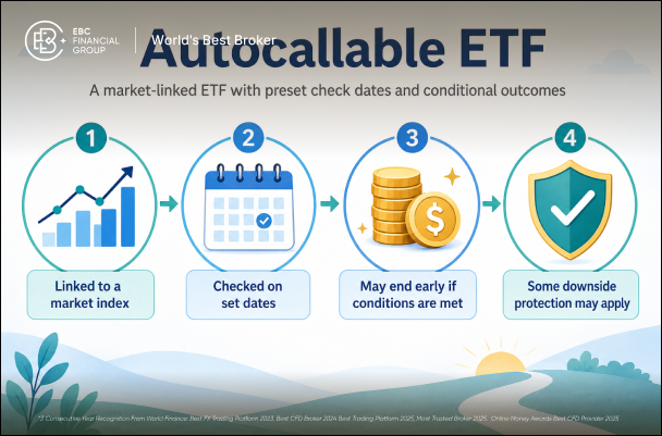
Autocallable ETFs bring structured-product mechanics into an exchange-traded fund, giving investors access to conditional payoff strategies without having to purchase individual autocallable notes directly. Many target relatively high distributions, while newer structures use similar mechanics to pursue long-term capital growth instead.
Understanding an autocallable ETF therefore requires looking beyond the headline yield or stated objective. The key questions are how the underlying payoff is structured, when positions can be called, what happens if markets fall, and how the ETF manages those exposures over time.
An autocallable ETF is an exchange-traded fund designed to provide exposure to autocallable strategies, typically linked to an equity index, basket of securities, or individual stock.
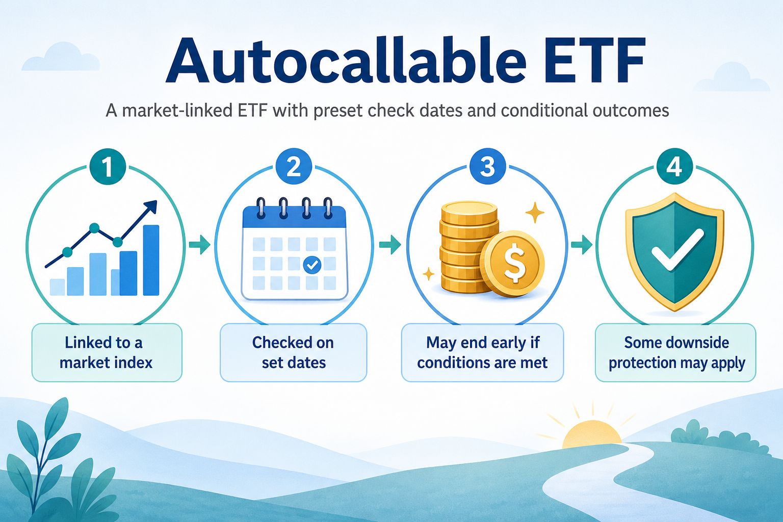
The word “autocallable” refers to the fact that the underlying structured position can terminate automatically when predetermined conditions are met. These conditions are usually based on the performance of a reference asset at specified observation dates.
Many autocallable strategies are built to generate conditional income while offering some degree of conditional downside mitigation. However, income is no longer a universal objective of the ETF category. The Calamos Autocallable Growth ETF (CAGE), launched on April 16, 2026, instead seeks long-term capital appreciation through laddered autocallable growth exposures with a memory feature. Coupons generated within its underlying synthetic exposures are reinvested rather than used to target regular income distributions.
This means “autocallable ETF” is better understood as a family of structured payoff strategies rather than a single standardized income product.
That makes an autocallable ETF fundamentally different from a traditional equity ETF. A conventional index fund typically aims to track the market. An autocallable ETF instead seeks to manufacture a defined or conditional payoff using structured exposures and derivatives.
The mechanics begin with a reference asset and an initial reference level. The strategy then defines a series of conditions that determine whether a coupon is generated, whether the position continues, and whether it is eventually called.
At specified observation dates, the reference asset is compared with predetermined thresholds.
If the underlying meets the autocall condition, the individual structured exposure terminates according to its terms. If the condition is not met, the position continues to the next observation date or ultimately to maturity.
The important distinction is that the ETF itself does not necessarily close when one position is autocalled.
An autocallable ETF may maintain several structured exposures at different stages of their life cycles. When one position is called, the fund can recycle the proceeds into a new exposure. This allows the ETF to remain continuously invested even though individual components may terminate along the way.
Before examining potential returns, several terms are important.
This is the index, stock, basket, or other market exposure against which the autocallable payoff is measured.
The starting value used to measure future performance of the reference asset.
An observation date is a predetermined point when the underlying is checked against the structure’s conditions. The outcome on these dates can materially affect returns.
This is the threshold that can trigger early termination of the structured exposure.
The coupon is the economic payoff generated within an autocallable structure when its required conditions are satisfied. It should not automatically be treated as the same thing as an ETF distribution.
An ETF distribution is the cash actually paid by the fund to shareholders. Its amount and tax character depend on how the fund implements the strategy, its expenses and its accounting. Some autocallable ETFs primarily use swaps rather than owning structured notes directly, and distributions can potentially include ordinary income, return of capital or both.
Some autocallables use a threshold that determines whether the coupon is generated at an observation date.
A separate barrier may determine whether an underlying autocallable receives its defined principal treatment at maturity or becomes exposed more directly to losses in the reference asset.
Crucially, this barrier is part of the payoff terms of the underlying autocallable exposure. It is not a floor beneath the ETF’s daily NAV or market price.
An ETF is continuously marked to market. Its value can therefore decline substantially before the underlying autocallables reach maturity, even if none ultimately breaches its maturity barrier. Someone selling ETF shares during that period may realise a loss without ever receiving the maturity outcome illustrated by the underlying structure. ProShares explicitly warns that its principal barriers do not protect the ETF itself from interim market declines.
Not every autocallable ETF uses the same combination of barriers, so the exact terms of each strategy need to be examined individually.
A current real-world structure helps illustrate how these thresholds interact.
The REX Autocallable Income ETF (ATCL) references a portfolio of synthetic autocallables with a 100% autocall level, a coupon barrier at 60% of the initial reference level and a maturity barrier at 50%. Individual exposures have five-year maturities and cannot be called during their first year. Coupon observations occur monthly, while autocall observations begin monthly after the one-year non-call period.
If the reference index is at or above 60% of its starting level at a coupon observation, the relevant autocallable can generate its coupon. If it falls below 60%, that period’s coupon is paused.
After the first year, an exposure can automatically terminate if the index is at or above 100% of its initial level on an autocall observation date.
If an exposure reaches final maturity without being called, the 50% maturity barrier becomes important. Finishing at or above that level allows the underlying structure to return principal according to its terms. Finishing below it exposes principal to the decline in the reference index.
These are ATCL’s specific parameters, not universal autocallable ETF rules. Other funds use different barriers, maturities, observation schedules and reference assets.
And again, ATCL’s 50% maturity barrier should not be interpreted as a 50% floor under ATCL’s ETF share price during the five-year life of those underlying exposures.
Autocallable income is generally created through options-based structured payoffs or derivatives that replicate similar economics.
The deeper economic explanation is that the structure is monetizing equity volatility while compensating the investor for accepting contingent income and nonlinear downside exposure.
Higher conditional coupons therefore do not represent free yield. They are linked to risks embedded in the payoff.
Volatility is particularly important. ProShares’ autocallable indexes target annualized volatility of 35% and can obtain leveraged equity exposure of up to 500% when measured volatility is low. ATCL references a volatility-managed equity index targeting 40%.
The amount of potential income therefore reflects more than ordinary option premium. The investor is accepting a payoff in which coupons may stop, upside can be constrained by autocall features, and sufficiently adverse market outcomes can result in substantial equity-linked losses.
Growth-oriented products can use the same underlying economics differently. CAGE, for example, uses a memory feature designed to retain missed coupons and capture them when conditions recover, with those economic payoffs reinvested to pursue compounding rather than regular income.
One of the important features of the ETF structure is the ability to spread autocallable exposures across different start dates and observation schedules.
Instead of relying on a single note, a fund can hold or replicate a ladder of autocallable positions. Each position may begin at a different time and reach its observation dates or maturity on a different schedule.
When one exposure is called, another may still be running. The proceeds from called positions can also be reinvested into new exposures.
Laddering therefore reduces the fund’s dependence on one specific entry point and removes some of the reinvestment burden associated with owning individual autocallable notes.
Importantly, there is no single standard laddering model. Existing U.S. autocallable ETFs already use materially different architectures.
| Example | Structure |
|---|---|
| CAIE | 52+ autocallables staggered weekly, five-year maturity, with coupon and maturity barriers 40% below the initial reference level |
| ATCL | Daily ladder of roughly 252 to 1,262 positions, 60% coupon level, 50% maturity level and five-year terms |
| ACSP, ACQQ and ACRT | Weekly issuance, three-year exposures, one-year non-call periods and 35% principal barriers |
| GraniteShares single-stock ETFs | Laddered autocallable exposure linked to individual stocks including Nvidia and Tesla |
| CAGE | Growth-oriented laddered autocallables with a memory feature and reinvestment rather than a conventional income objective |
This diversity is why an autocallable ETF should be viewed as a family of payoff architectures rather than one standardized product.
The ETF wrapper changes how investors can access the strategy.
Individual structured notes may involve higher investment minimums, limited secondary-market liquidity, and the need to reinvest manually when a note is called or matures.
An ETF can offer exchange trading, continuous portfolio management, and exposure to multiple structured positions within a single fund.
The wrapper may also alter the nature of credit exposure. Holding an individual structured note can involve direct exposure to the issuer’s creditworthiness. An ETF may reduce that specific concentration, although derivative-based strategies can still introduce counterparty risk.
The ETF structure therefore improves accessibility and implementation, but it does not remove the risks embedded in the autocallable payoff.
One of the easiest mistakes is to compare an autocallable ETF’s headline distribution rate directly with a bond yield.
They are not equivalent measurements.
First Trust’s FT Vest Laddered Autocallable Barrier & Income ETF (ACYN) provides a useful example. As of August 31, 2026, First Trust reported a 10.01% distribution rate but a 2.88% 30-day SEC yield. The fund had approximately $1.79 billion in net assets as of September 1.
There is no contradiction between those figures. They measure different things.
A distribution rate annualizes recent cash distributions relative to the fund’s price or NAV. The SEC yield uses a standardized calculation intended to measure income earned over a specified period after expenses. Neither should automatically be equated with the coupon embedded in the underlying autocallable structure or with the shareholder’s eventual total return.
The useful distinction is:
headline distribution rate ≠ underlying autocallable coupon ≠ SEC yield ≠ total return.
A fund can make a large distribution while its NAV declines. Depending on the fund, distributions may also include return of capital. Looking at the headline percentage alone therefore provides an incomplete picture of economic performance.
The most important risk is a severe decline in the reference asset.
Barrier features may provide conditional downside mitigation to the underlying autocallable payoff, but they do not guarantee that an ETF shareholder’s losses are limited to the barrier level. A 50% maturity barrier, for example, does not mean the ETF itself has 50% downside protection.
The barrier determines the treatment of an underlying autocallable at the relevant observation or maturity date. The ETF’s NAV and market price remain exposed to changing market valuations throughout the holding period.
Autocallable ETFs can also limit upside. If markets rally strongly, income-oriented investors may receive the defined payoff while missing part of the appreciation that would have been captured by owning the underlying asset directly.
Path dependency adds another layer of complexity. Returns can depend not only on where the market finishes, but also on where it trades on specific observation dates.
There is also distribution risk because coupons and shareholder distributions may be conditional or variable. Derivatives can introduce counterparty and valuation risk, while ETF shares can trade at a premium or discount to net asset value during stressed markets.
Volatility-managed reference indexes can create additional risk. Strategies that increase equity exposure when measured volatility is low can subsequently experience amplified moves if market conditions change quickly.
Finally, complexity itself is a risk. Two autocallable ETFs may use materially different barriers, observation schedules, reference assets, volatility targets, laddering methods or replication structures even if their headline objectives appear similar.
Covered-call ETFs are a particularly useful comparison because both strategies may be used to pursue high equity-linked income, but they obtain that income differently.
| Feature | Autocallable Income ETF | Covered-Call ETF |
|---|---|---|
| Income source | Conditional structured payoff linked to accepting downside risk | Premium from selling call options |
| Upside | Generally constrained by autocall and payoff terms | Partially or substantially surrendered through sold calls |
| Downside | Can become strongly equity-linked when maturity barriers are breached | Generally participates in underlying losses, partly offset by option premium |
| Path dependency | Depends heavily on barriers, observation dates and autocall conditions | Driven mainly by underlying performance and the option-writing cycle |
Covered-call ETFs primarily monetize part of the market’s potential upside through call-option premiums. Autocallable income strategies instead generate their economics through predefined conditional payoffs in which the investor accepts downside-linked risk.
Neither structure eliminates equity risk, and comparing their distribution rates alone can obscure the very different risks used to produce those distributions.
Their performance can vary substantially depending on both the market environment and the structure being used.
In a rising market, an income-oriented autocallable position may be called relatively quickly. The defined payment can be generated, but further upside may be sacrificed if the market continues climbing.
In a sideways or moderately declining market, an income strategy may continue generating coupons as long as the relevant conditions remain satisfied.
A sharper decline can change the outcome. Coupons may stop if a coupon barrier is breached, while a sufficiently large fall at the relevant maturity test can expose the underlying autocallable to substantial losses.
Growth-oriented structures can behave differently. A memory feature may preserve missed economic coupons for potential capture following a recovery, while reinvestment changes the objective from current income toward longer-term compounding.
For this reason, the behaviour of an autocallable ETF cannot be inferred from the word “autocallable” alone. Its objective and precise payoff architecture have to be examined first.
The stated distribution rate should only be the beginning of the analysis for an income-oriented fund, while growth-oriented products require the same scrutiny of their underlying payoff mechanics.
Investors should examine the reference asset, initial reference level, autocall threshold, coupon conditions, downside barriers, observation schedule, maturity terms, volatility target and maximum potential loss.
It is also important to understand whether the ETF holds structured exposures directly or uses derivatives such as swaps to replicate them.
Fees, liquidity, bid-ask spreads, counterparty exposure, the treatment of called positions and the source and tax character of distributions can also affect the investment experience.
Most importantly, investors should distinguish the payoff generated inside an autocallable exposure from the return earned by an ETF shareholder. A high coupon or distribution does not necessarily translate into a strong total return if the ETF’s net asset value declines.
Autocallable ETFs package complex structured-payoff strategies inside an exchange-traded fund. Many seek conditional income, while newer products show that the same framework can also be adapted for long-term growth through features such as coupon memory and reinvestment.
The trade-offs depend on the architecture. Income may be conditional, upside can be constrained, volatility can amplify both the potential payoff and the risk, and sufficiently adverse market outcomes can lead to substantial losses.
Most importantly, a maturity barrier should never be mistaken for a floor beneath an ETF’s daily value, while an advertised distribution rate should not be confused with an underlying coupon, SEC yield or total return.
For that reason, evaluating an autocallable ETF should begin with its payoff structure rather than its headline distribution or objective. Understanding the reference asset, observation dates, autocall conditions, barriers, volatility exposure and implementation method provides a much clearer picture of how the strategy works and what risks are being taken.